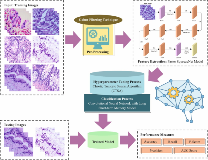
This article introduces the PACHS-DLBDDM methodology. The proposed methodology focuses mainly on the recognition and classification of LCC. It comprises GF, Faster SqueezeNet, CNN-LSTM, and CTSA techniques for preprocessing, feature vector generation, classification, and hyperparameter tuning processes. Figure 1 depicts the entire flow of the PACHS-DLBDDM technique.

Overall flow of PACHS-DLBDDM methodology.

Image preprocessing

At the primary stage, the PACHS-DLBDDM technique employs GF to preprocess the input images²⁶. The GF model is utilized for its efficiency in capturing texture and spatial frequency data, which is significant for evaluating medical images where subtle patterns are crucial. GF method outperforms edge detection and texture characterization, allowing it to accentuate significant features in complex images like those employed for cancer detection. Its capability to filter images with several orientations and scales makes it proficient in discriminating between fine details and noise. This capability safeguards robust preprocessing, improving the accuracy of subsequent feature extraction and classification steps. Furthermore, GF’s well-established mathematical foundation and ease of implementation contribute to its dependable performance across diverse imaging modalities. Figure 2 demonstrates the structure of the GF model.

Overall structure of GF technique.

GF is a popular image preprocessing method applied in medical imaging for LCC recognition. It includes applications of GF to emphasize specific characteristics in medical images, including edge and texture information. GF improves the visibility of tumour structure by filtering images at varying orientations and scales, making detecting malignant areas simple. This technique optimizes the performance of succeeding image analysis and classification methods. The ability of GF to highlight pertinent features assists in earlier detection and treatment planning for LCC patients.

Faster SqueezeNet model

Next, the PACHS-DLBDDM approach employs the Faster SqueezeNet to generate feature vectors²⁷. Faster SqueezeNet is selected for feature vector generation due to its efficient balance between model size and performance. Its compact architecture safeguards fast processing and low computational cost, making it ideal for real-time applications with substantial rapid feature extraction. Despite its small size, SqueezeNet maintains high accuracy in capturing relevant features, which is crucial for precise classification and evaluation. The reduced memory footprint of the technique allows for deployment on devices with limited resources, improving its practical usability. Furthermore, Faster SqueezeNet’s pre-trained models present robust feature extraction capabilities, utilizing extensive training on large datasets to enhance generalization across diverse tasks.

The SqueezeNet architecture was introduced, which has fewer parameters while retaining the performance since AlexNet and VGGNet parameters are ever-increasing. The primary foundation in SqueezeNet is the Fire model. This is broken down into Squeeze and Expand models. Squeeze comprises \(\:S1\)×\(\:1\) convolutional kernels. The Expand layer has \(\:1\)x\(\:1\) and \(\:3\)x\(\:3\) convolutional layers. \(\:{E}_{1\times\:1}\) and \(\:{E}_{3\times\:3}\) are the number of \(\:1\)×\(\:1\) and the count of \(\:3\)×\(\:3\) convolutional layers\(\:.\) This method should satisfy \(\:S<\left({E}_{1\times\:1}+{E}_{3\times\:3}\right)\).

The \(\:\text{M}\text{i}\text{n}\) uses an MLP rather than the linear convolutional layer to improve the network performance. The MLP corresponds to the cascaded cross-channel parametric pooling layer, accomplishing an information integration and linear combination of feature maps.

Once the input and output channels are larger, the convolution layer develops superiorly. A \(\:1\)x\(\:1\) convolutional layer has been added to the inception module, reducing the number of input channels and decreasing the operation complexity and convolution layer. Finally, a \(\:1\)x\(\:1\) convolutional layer is added to enhance feature extraction and increase the number of channels.

SqueezeNet is used to replace \(\:3\)×\(\:3\) with \(\:1\)×\(\:1\) convolutional kernels to reduce the parameter. Once the sampling reduction function is delayed, the convolutional is given a large activation graph; however, the large activation preserves further details, providing a high classifier performance.

Fast SqueezeNet is introduced to improve performance. Residual and BatchNorm designs are included to avoid overfitting. It is the same as DenseNet.

Faster SqueezeNet includes four convolution layers, a global pooling layer, 1 BatchNorm layer, and three block layers.

Fast SqueezeNet is given as follows:

1. (1)

   It is derived from the DenseNet architecture, and a connection method has been developed to improve data flow between layers. This includes a pooling layer and a fire module. Lastly, the two concat layers are linked to the next convolution layer. The current layer obtains the mapping feature of the previous layer and applies \(\:{x}_{0},\dots\:,{\:and\:x}_{l-1}\) as input.

In Eq. (1), \(\:[{x}_{0},\:{x}_{1},\:\dots\:,\:{x}_{l-1}]\) denotes the feature map connection at \(\:\text{0,1},\dots\:,l-1\) and \(\:{H}_{l}\) concatenate various inputs. \(\:{x}_{0}\) is the \(\:\text{m}\text{a}\text{x}\)-pooling layer, \(\:{x}_{1}\) is the Fire layer, and \(\:{x}_{l}\) denotes the concat layer.

1. (2)

   It is learned from the ResNet design, which includes a fire module and pooling layer to ensure better convergence. Finally, it is connected to the next layer after the two layers are summed.

In ResNet, the shortcut connection applies an identity map directly, signifying that the convolution input has been added straightaway to the output. \(\:H\left(x\right)\) denotes the desired underlying mapping. A stacked non-linear layer fits an alternative mapping of \(\:F\left(x\right):=H\left(x\right)-x.\) A novel mapping is changed into \(\:F\left(x\right)+x.\) The shortcut connection skips multiple layers. As a result, the ResNet model is used to resolve the degradation and vanishing gradient problems without increasing the network parameter.

Classification method using CNN-LSTM

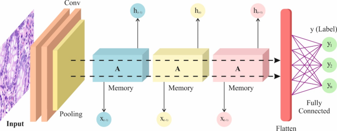
During this stage, the CNN-LSTM approach has been used for LCC classification²⁸. Assuming the spatial feature extractor benefits of the convolution (Conv) layer of CNN and the time-based forming benefits of the LSTM method, this research develops CNN-LSTM that can depict the local feature and retain the long-term dependencies. The CNN-LSTM technique is selected for LCC classification due to its prevailing integration of spatial and temporal feature extraction abilities. The CNN technique outperforms in precisely detecting spatial patterns and textures within images, making them appropriate for extracting detailed features from lung cancer cell images. By incorporating the LSTM networks, which are proficient at capturing temporal dependencies and sequential patterns, the technique can efficiently manage and analyze time-series data or sequential image features, enhancing the accuracy of the classification. This hybrid technique employs the proficiency of the CNN model in feature extraction and the strength of LSTM in sequence learning, giving an overall examination of the cancer cells. It improves the capability of the technique to detect complex patterns and discrepancies over time, paving the way to more precise and reliable LCC classification.

On input to the CNN-LSTM method, which consecutively crosses over Conv block1 and Conv block2, it results in output sizes of \(\:(64,\:26,\:26)\) for Conv block1 and \(\:(128,\:13,\:13)\:\)for Conv block2. Every Conv block has a batch normalization (BN) layer, a Conv layer, ReLU, a dropout layer, and a pooling layer. The BN layer hastens the training and recovers the generality capability of the method. The ReLU relates non-linearity and sparsity to configuration and averts the gradient from vanishing. The ReLU activation function calculation is as follows:

The pooling layer used the largest size of \(\:2\text{x}2\), efficiently decreasing the parameter of model and memory desires; the dropout layer with a definite prospect throughout the system training procedure improves the model’s generality skill. Subsequently, the related features removed by CNN are served into the dual-layer LSTM model to get every time-based feature. The 1st layer LSTM contains 100 HLs, and the 2nd layer LSTM contains 50 HLs. The three gates are accessible in every LSTM framework, with forget, input, and output gates. Figure 3 illustrates the structure of CNN-LSTM.

Architecture of CNN-LSTM.

The LSTM defends and handles the cell state over three gates, recognizing the forgetting, long-term remembering, and state upgrading. The interior processing of LSTM has been calculated as below:

Whereas \(\:{f}_{t},{\:i}_{t}\), and \(\:{\text{o}}_{t}\) signify the gates of forgetting, input and output, correspondingly; \(\:{c}_{t}\) refers to the internal state, which removed from \(\:0\sim\:t\) time denotes the transporter of long-term memory; \(\:{b}_{f},{\:b}_{i},{\:b}_{\text{o}}\), and \(\:{b}_{C}\) denotes the biases; \(\:{h}_{t}\) signifies the long and short-term memory output at the moment \(\:t\); \(\:\left[{W}_{fx},{\:W}_{fh}\right],\left[{\:W}_{ix},{\:W}_{ih}\right],\left[{\:W}_{ox},\:{W}_{oh}\right]\), and \(\:\left[{W}_{\stackrel{\sim}{c}x},\:{W}_{\stackrel{\sim}{c}h}\right]\) represents the weights of forget, input, output gates, and the unitary input, correspondingly; and \(\:\sigma\:\) indicates an activation function of sigmoid.

Fine-tuning the DL model

As a final point, the CTSA approach is performed to enhance the hyperparameter value of the CNN-LSTM model. TSA denotes a novel meta-heuristic technique stimulated by swarm intelligence (SI)²⁹. The CTSA is selected for its greater performance in hyperparameter tuning and optimization due to its capability to escape local optima and explore the solution space more thoroughly. Unlike conventional techniques, the CTSA model utilizes chaotic sequences to improve randomness and avoid premature convergence, which is significant for complex models with high-dimensional parameter spaces. This paves the way for more precise parameter settings and enhanced model performance. Furthermore, CTSA’s integration of swarm intelligence and chaotic behaviour results in improved convergence rates and robustness compared to other optimization methods, making it highly efficient for fine-tuning the classification procedure in cancer detection systems. Its adaptability and efficiency are crucial in optimizing complex techniques and attaining high classification accuracy.

Tunicate is a horde that mainly hunts for its food resources in the ocean. SI and Jet propulsion are the dual dissimilar conducts of tunicate. The 3 phases of the jet propulsion performance are described below. At first, they evade crashes among the hunting agents. Then, they travel to the optimal search agent location. At last, they stay nearer to the optimal searching agent. It upgrades the other searching agents to a superior solution.

The \(\:\overrightarrow{A}\) vector is employed to compute the upgraded position of searching agents to avoid crashes among search agents:

Here, the water movement advection is denoted by \(\:\:\overrightarrow{F}\), and \(\:\overrightarrow{G}\) represents the gravity force. \(\:{c}_{1},{c}_{2}\) and \(\:{c}_{3}\) signify the variables within the range of \(\:\left[\text{0,1}\right].\)\(\:\overrightarrow{M}\) indicates the social force among the search agents as given below:

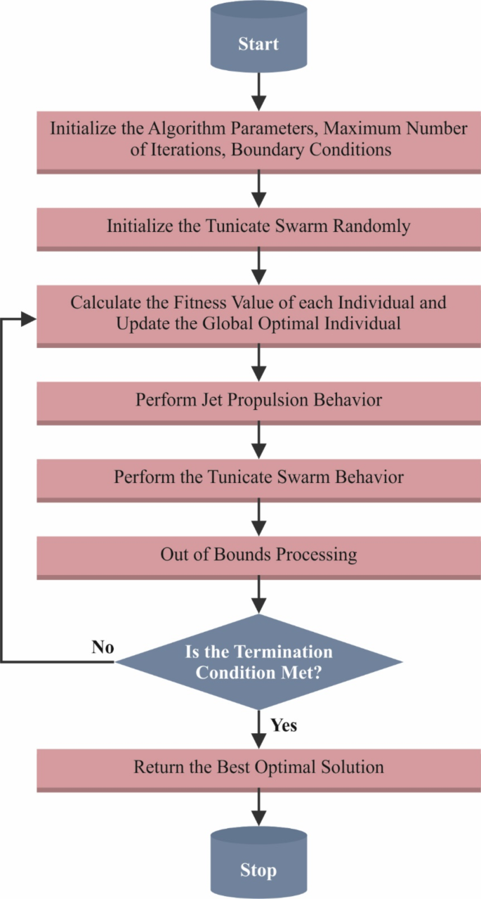
\(\:{P}_{\text{m}\text{a}\text{x}}\) and \(\:{P}_{\text{m}\text{i}\text{n}}\) represent the ^first and ^second velocities for creating social communication, respectively. The \(\:1\) and \(\:4\) are fixed values. Figure 4 depicts the architecture of the CTSA model.

Architecture of CTSA model.

The searching agent moves to the finest neighbour way after avoiding the crash among adjoining locals. The mathematical calculation of this method is given below:

Where\(\:\:\overrightarrow{P}D\) indicates the distance between the source of food and the search agent, viz., tunicate, \(\:F\overrightarrow{S}\) epitomizes the position of the food source. \(\:{\overrightarrow{X}}_{i}\left(t\right)\) signifies the position of the tunicate, and \(\:rand\) denotes the random integer in the range of [0 and 1].

The agents uphold the position near the optimal searching agents is stated as below:

In Eq. (14), \(\:\overrightarrow{X}\left(t\right)\) displays the tunicate position after upgrading \(\:the\:F\overrightarrow{S}\) position. The initial dual optimal solutions are kept and upgraded with other searching agents depending upon the optimal searching agent’s place to demonstrate the tunicate’s group behaviours arithmetically.

Initialization of population is crucial in meta-heuristic techniques since the excellence of solution and velocity of convergence are influenced by it. So, the initialization of the population is produced at random because there is no preceding knowledge accessible for the solution, and it is frequently used in meta-heuristic techniques. Likewise, TSA exploits the early arbitrary population of \(\:X\) utilizing normal distribution as set below:

In Eq. (16), \(\:{x}_{ij}\left(t\right)\) denotes the \(\:jth\) module of\(\:\:ith\) individual solution at \(\:th\) iteration\(\:.\) The search region’s upper and lower limits are \(\:{x}_{\:\text{m}\text{a}\text{x}}\) and \(\:{x}_{m\dot{m}},\:\)respectively. \(\:r\) signifies the random value in the range of [\(\:\text{0,1}\)].

If the initialization of the population is nearer to the global targets, the rate of convergence turns fast, and it can achieve improved solutions; however, the early population is less frequently the finest randomly. The chaotic-based method enhances efficiency and improves the variety of the population.

In Eq. (17), \(\:c{h}_{ij}\) denotes the value of chaotic that is formed by the logistic chaotic mapping:

The OBL technique computes the reverse solution \(\check{X}\) of \(\:{X}_{i}\). The \(\:n\) best solutions were selected from \(\:[X,\:x]\) as per the fitness value. Eventually, the technique drives to the phase of jumping.

The CTSA model develops an FF to improve the classifier’s effectiveness. It designates an optimistic numeral to signify the candidate solution’s amended performance. In this paper, the reduction of the classifier’s rate of error is measured as FF, which is shown in Eq. (19).